Profiling in PyTorch (Part 2): From nn.Linear to a Fused MLP

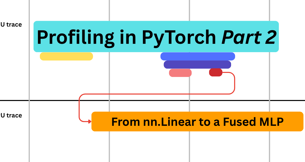
Hugging Face outlined updates on Profiling in PyTorch (Part 2): From nn.Linear to a Fused MLP: profiling in PyTorch (Part 2): From nn.Linear to a Fused MLP

Can –compile help a single Linear? Where did the transpose go? Kernel layouts and pre-ops Stacking three Linears: the MLP Why are there two types of GEMM kernels? What does torch.compile do? The fused Triton kernel Let's use hand tuned kernels Why use the kernels library Why tuned kernels are better Conclusion This is the second post of Profiling in PyTorch, a series where we slowly build the skill of reading profiler traces and use it to drive optimization: In the first part of this series “Profiling in PyTorch”, we used torch.add(torch.matmul(x, w), b) to learn how to read PyTorch profiler traces. We also discussed several other topics that came our way – the CPU dispatch chain, launch overhead, the difference between an overhead-bound and a compute-bound regime, and some internals of torch.compile. In the second iteration (this blog post), we climb one rung up the ladder. We replace the hand-written matmul-add pair with an nn.Linear (with bias=True). This is the building block every deep learning model uses. We then stack three of them (specific to our example), with an activation in between, to form a Multilayer Perceptron (MLP) block. The scripts for this blog post live here: 02_linear.py, 03_simple_mlp.py, and 03_kernels_mlp.py. Like before, it helps to open them in a separate tab and walk through the code as you read. We use an NVIDIA A100-SXM4-80GB GPU to run the scripts. It is really easy to set up a GPU on the Hugging Face infrastructure and experiment with the scripts using Dev Mode with Spaces. One could also run the scripts with the Hugging Face Jobs pipeline.